To recap - in the last blog post we talked about how to find recordings in State Library of Queensland's collections, some heuristics for evaluating audio quality. and where we can use State Library’s resources. Parallel to this process I've been researching the datasets used to train speech synthesis models - specifically text to speech (TTS), aiming to pick a dataset format that is relatively simple to implement and widely used. This will enable enable re-use of the same dataset across various model training systems, and allowing a bit of wriggle room when it comes actually implementing models
The key resources for this are:
-
paperswithcode.com a site dedicated to the latest research in machine learning with actual working code examples
-
github, where most of the code repositories can be found with its easily searchable tagging system
-
huggingface.co hosts one of the largest and most popular repositories, with
-
and of course - your friend and mine chatgpt - the expert that never tires of answering dumb questions.
After much research, I settled on the LJ Speech dataset format. The original dataset in this format was produced around 2016 from public domain recordings, and the format is widely used in speech synthesis libraries.
An LJ Speech dataset consists of a metadata.csv file and a folder with audio files in the wav format. These files are mono, with a sample rate of 22050khz at 16bits. Each audio file needs a corresponding line in the metadata.csv that has the name of the file, and the text content spoken. This text should be normalised, meaning numbers and abbreviations should be spelt out in full.
As we prepare our LJ Speech format dataset(s), lets go through a few examples of what we've found in the collections, and introduce some programmatic tools that we can use to speed-up our data processing. Its also worth spending some time understanding why we'd use these tools instead of the recording studio software.
Although the audio applications mention previously are state-of-the-art, and we can also use them to perform the tasks required to create datasets, we have a problem : machine learning models generally require lots and lots of labelled data. Applications used in recording studios are used to create bespoke audio outputs - think mixing multiple tracks together to mix a pop song or video soundtrack, or carefully editing a podcast recording. The files used may be large - tens or hundreds of megabytes, but the outputs are generally speaking, relatively short in duration, and are a single contiguous files with a simple label or name. Machine learning (ML) audio datasets are large in aggregate, gigabytes in size, but are generally made of smaller files along with a separate metadata file that describes the dataset in terms relevant to the model being trained. The metadata can be generated by another ML tool – used to transcribe or analyse. ML tools can also be used to ‘augment’ the data, modifying existing data using signal processing techniques to generate variations.
The key takeaway is that despite being audio, ML audio datasets are not made for people to listen to, rather for ML systems to ingest, process, transform and use generatively. Small changes (or mistakes) in a dataset can have significant impacts on the quality or viability of the model being trained, so we want a system we can use iteratively -over and again, to refine our dataset without having to spend the time reconstructing systems from raw files.
Most of the tools for the job of preparing datasets are part of the giant ecosystem of the programming language python https://www.python.org/ . The popularity of python in ML research means we can find an automated way of doing just about any task required, again github is where many of these projects are found, and gpt4 is the perfect programming assistant to join these tools together into scripts.
From these examples, and knowing our targeted dataset format we can build up a workflow using a combination of manual processing using audio apps and python scripts to wrangle our data into shape. The basic steps are:
-
Audio analysis (manual + automated)
-
Initial processing (manual)
-
dataset generation (automated)
-
transcription with timestamps
-
split into sentences
-
metadata.csv generation
-
with text normalised
-
-
Audio processing
Audio Analysis
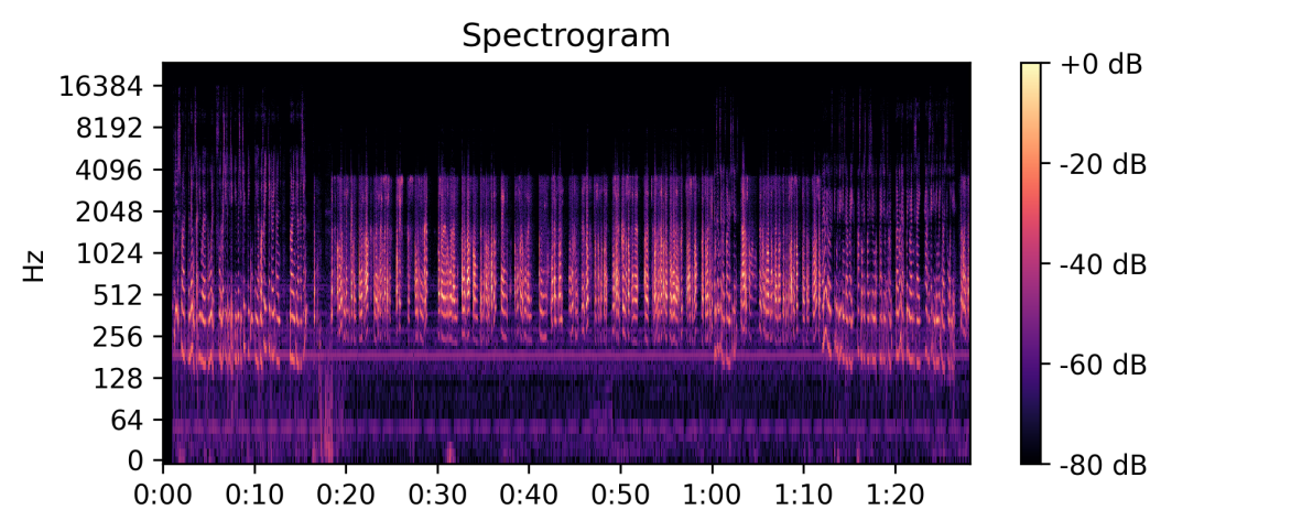
Our first example comes from Acc 32233, Five Years On: Toowoomba and Lockyer Valley flash floods: oral history interviews. These oral histories are enthralling stories, and speak to the tragedy and turmoil of that event and the resilience of those who lived through it. Some of the oral histories in this collection are recorded with the interviewee on a telephone, with a limited bandwidth and distortion. Our ears easily understand and follow these stories, but for a dataset we are after higher fidelity. Rather that open each file and listening for changes in audio quality (in this case bandwidth), we can use a python library (a collection of software) called librosa to visualise this. On the left had side we have a frequency scale, with time from left to right along the bottom. We can clear see how the highest frequency drops from about 16,000 hz, to 4000 hz, indicating a significant drop in audio quality. A simple python script lets us run this analysis on all our downloaded collections.
Manual audio analysis
While automated analysis is perfect for narrowing down our broad selection, some subtle issues are still difficult to detect programmatically. An example can be found in Acc 28839 Our Rocklea: connecting with the heart through story and creativity 2012. Automated analysis of this dataset will likely miss the high frequency artefacts present on the left channel in part 2 of Marion Braund’s story. . These crackles are obvious to the ear, and the easy fix is to discard the left channel and work with the right channel only at the initial processing stage.
Initial processing
With our audio files analysed and some decisions made we can do some initial processing on entire audio files using izotope RX. RX has a powerful suite of audio restoration tools, that with some tweaks of the settings can product excellent results. For example in TR 1859, Peter Gray Audiotapes, we have a mono audio file originally recorded on a reel-to-reel analog audio tape (hence the limited bandwidth), then digitised at 44,100 khz. In the highlighted section just noise is present:
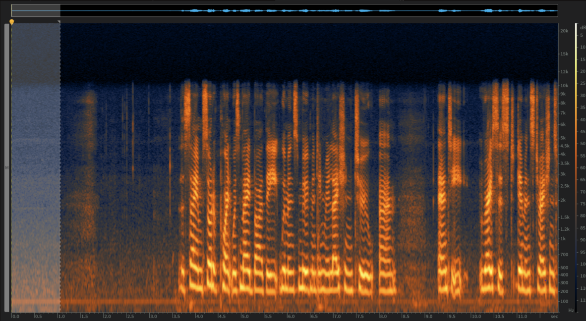
This noise profile can be learnt in the spectral de-noising module (the noise profile is orange).

Then used judiciously to remove this noise from the audio file.
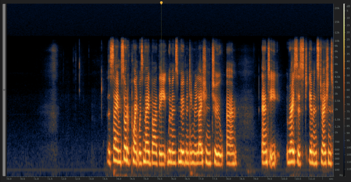
The removal of noise can reveal or make more obvious other artefacts, in this case there is low frequency hum present at about 100 hz (marked in red), and some extraneous “mouth noise” (in green).

A simple high-pass filter will get rid of the former, and the later can be considered a natural part of speech and safely ignored.
Dataset generation
With our selection and initial processing complete – its time to generate our dataset. The first step in this process is transcription of the audio file, to produced a diarized, timestamped transcription. Diarization is the process of identifying and labelling each line of a transcript with a speaker ID, timestamps means each line has a start and end time, usually in minutes and seconds.
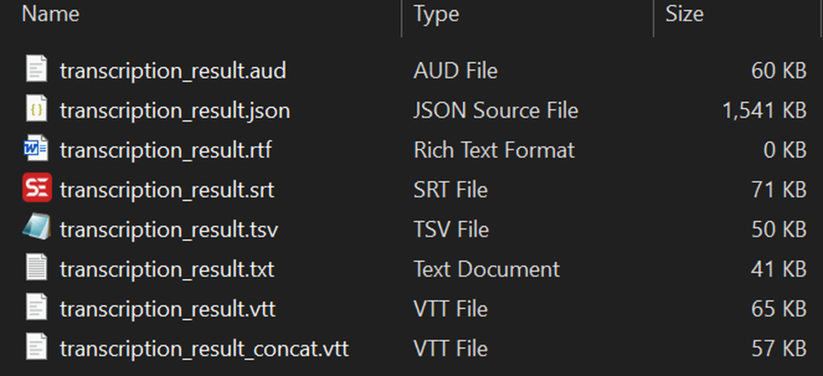
We will use a version of the remarkable whisper automatic speech recognition (ASR) system for this. WhisperX achieves up to 70x faster than real-time transcription as well as annotating output with speaker ID labels for diarization with pyannote-audio . WhisperX outputs various subtitle formats, as well a JSON file that contains word-level time stamps that come in handy if we want to make more detailed processing.
The webvtt output for a transcript looks something like this:
WEBVTT
00:01.141 --> 00:05.625
[SPEAKER_01]: This is an interview with Sharon Poulsland at Spring Bluff.
00:05.625 --> 00:16.694
[SPEAKER_01]: It's the 26th of May, 2016, five years after the disaster which came through Spring Bluff and Toowoomba and the Lockyer Valley.
00:16.694 --> 00:19.756
[SPEAKER_01]: Thank you very much, Sharon, for speaking to me today.
00:19.756 --> 00:21.297
[SPEAKER_00]: My pleasure.
00:21.297 --> 00:30.785
[SPEAKER_01]: Five years on from the disaster, could you give me a brief description of what's happened for the community of Spring Bluff and the recovery?
00:35.505 --> 00:38.546
[SPEAKER_00]: It's been a lot of hard work, I guess.
00:38.546 --> 00:43.448
[SPEAKER_00]: Spring Bluff became, with Murphys Creek I guess, a bit of us and them.
00:43.448 --> 00:48.309
[SPEAKER_00]: We were certainly held at arm's length by Murphys Creek and we don't belong
From the webvtt file we can produce both our metadata.csv and split our audio file into sentences, each correctly labelled and output to a folder. As the oral histories usually have an interviewer audible in the file, we will get a metadata.csv and folder of audio files for each. Here is the metadata file from SPEAKER_00 in the format “segment_id|text|normalised text
Segment_1| It's been a lot of hard work, I guess.| It's been a lot of hard work, I guess.
Segment_2| Spring Bluff became, with Murphys Creek I guess, a bit of us and them.| Spring Bluff became, with Murphys Creek I guess, a bit of us and them.
Segment_3| We were certainly held at arm's length by Murphys Creek and we don't belong.| We were certainly held at arm's length by Murphys Creek and we don't belong.
Segment_4| I remember going to one of the council community meetings for, you know, what can we do better in the future and how can we plan better and that sort of thing.| I remember going to one of the council community meetings for, you know, what can we do better in the future and how can we plan better and that sort of thing.
And SPEAKER_01 output looks like this:
Segment_1| This is an interview with Sharon Poulsland at Spring Bluff.| This is an interview with Sharon Poulsland at Spring Bluff.
Segment_2| It's the 26th of May, 2016, five years after the disaster which came through Spring Bluff and Toowoomba and the Lockyer Valley.| It's the twenty-sixth of May, two thousand and sixteen, five years after the disaster which came through Spring Bluff and Toowoomba and the Lockyer Valley.
Segment_3| Thank you very much, Sharon, for speaking to me today.| Thank you very much, Sharon, for speaking to me today.
Looking at Segment_2 for SPEAKER_01 we can see the result of text normalisation using Ljnormalize. Numbers are written out – eg “26th of May” becomes “twenty-sixth of May”.
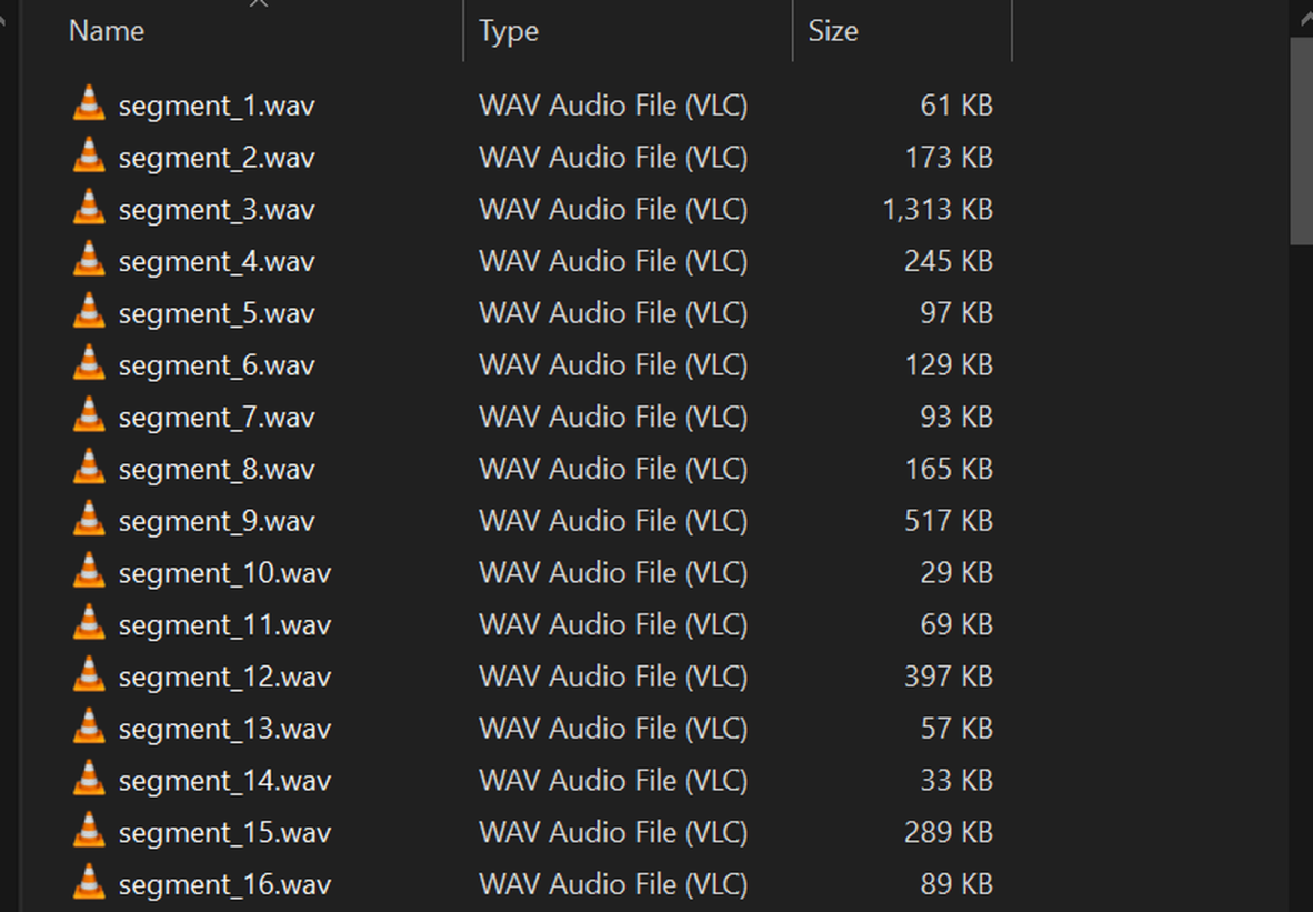
At the same time as producing the metadata.csv, we can use the same information to split the long audio file into single lines using the python FFMPEG library. We’ll end up with a folder containing our metadata.csv, and our wav folder.
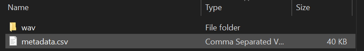
And inside the wave folder we have our named audio files
Audio processing
The final step is to convert all our segments to mono, downsample and normalise the audio level. The best tools for the this job are the librosa library mentioned earlier, and SoX a cross platform audio processing program which can be used in python via a wrapper. SoX provides high quality resampling, ensuring that our final audio files are free from processing artifacts.
Final Thoughts
With a workable pipeline, we are ready to create our datasets. No doubt this pipeline will require tweaks once we start testing and training models, but being mainly programmatic in nature we can test and apply changes as we go.
Comments
Your email address will not be published.
We welcome relevant, respectful comments.